Chapter 5 Analyzing the Data

5.1 Basic steps when analyzing the data
Think again about your research question and what you are trying to learn or discover. How can you use your data to answer this question?
The data to be analyzed should correspond to the core elements of the hypothesis to be investigated. You investigate whether the postulated cause-effect relationship exists, or quantitatively identify the strength of the effect. To perform a reproducible research project you need to generate an analysis dataset. For information on how to generate an analysis dataset and how to create a set of programs that describes how the secondary data used are synthesized, processed and analyzed, go to Basic steps when processing and preparing the data.
Using your analysis dataset you perfrom two more steps to examine your research question. Across both steps, try to use data visualization with tables and graphs. They are an essential part of your work. Visualizations help to support the argumentation in the text and visualize complex facts in a simple form.
In the following, we describe the two major tasks for data analysis
- Describe your data, assess validity and plausiblity
- Generate estimates of your investigated effect using regression techniques
5.1.1 Describe your data, assess validity and plausiblity
Start the data analysis by doing some descriptive analyses of your data and sample. Once you have selected the necessary variables, generated new variables for the analysis, and combined all the necessary datasets into one analysis dataset you can start your empirical investigation.
- Check the plausibility by looking at basic descriptives (N, mean, median, frequencies)
- Plot the distribution of your data using histograms, boxplots, bar charts
- Critically reflect any anormalities: Compare your data with the reference literature
- Are descriptives similar? If not, why so? Try to assess coding problems, different population, unbalanced samples.
5.1.2 Generate estimates of your investigated effect using regression techniques
Once you have decided on the type of empirical analyses you would like to perform, run the regressions.
Perform the regression analyses. That means use the appropriate procedure to estimate regressions that reflect your empirical strategy.
Create output tables that report your results which outsiders can understand. Label your variables properly.
Concentrate on analyzing and interpreting the effects of your variable of interest (\(X\))
- interpret and show in tables only most important and relevant coefficients related to the research question. For example, you do not need to interpret and display coefficients for all of the incuded control variables, just the main variables of interest.
Think about how to interpret your estimates.
Challenge your approach. Investigate why your estimates might not be plausible.
Again, compare with existing literature.
What do your data say? After you run the regressions, look at the results:
- Are your main coefficients of interest statistically significant: is the p-value smaller than 0.05 or any other pre-defined level of significance?
- Consider also the economic significance of your results. Is the effect you are measuring large or small?
- Do your results make sense or are they counterintuitive? This might give you a clue that you might have misspecified your regression or made a mistake in your analysis.
5.2 Resources box
Repositories of statistical techniques, including data wrangling
Data Analysis
- Princeton University Library: Getting Started in Data Analysis using Stata and R
- Data Analysis for Business, Economics, and Policy
Organizing your workflow, programming and automation
- Gentzkow M, Shapiro J. Code and Data for the Social Sciences: A Practitioner’s Guide [Internet]. Chicago Booth and NBER; 2014
- The Stata workflow Guide
- In Stata coding, Style is the Essential: A brief commentary on do-file style
Data Visualization
- The chapter Data Visualization Basics by Hans Sievertsen includes important resources for the fundamentals of data visualization
- Stata Cheat Sheet on Visualization provides an overview of the technical implementation
- Jones AM. Data visualization and health econometrics. Foundations and Trends in Econometrics. 2017
Create journal submission-ready output tables
5.3 Checklist to analyzing the data
- Follow your research question and hypothesis. Do not alter it while analyzing the data.
- Do your results make sense? If not, rule out any programming errors.
- Try to interpret your results. How big is your effect? Is it small or large?
- Use visualizatoin techniques as often as possible to analyze your data.
- Discuss your results with your supervisor, colleagues or fellow students.
5.4 Example: Hellerstein (1998)
Hellerstein’s 1998 study aims to identify the role the physician plays in prescribing a generic over a trade-name drug and the role of a patient’s insurance status. To identify this, we analyze the secondary data on physician level in cross-sectional format (NAMCS and NAMCSd, described in the chapter “running the study and collecting the data”). The primary interest is to investigate if physicians do or do not prescribe a generic drug and whether this is influenced by the patient’s insurance status. We are not investigating prescription behavior of physicians over time using panel data.
Over the course of the analysis, we want to explore the dataset. This includes describing and assessing its validity and plausibility. Thus, before generating estimates of the effect of interest using regression techniques, we describe the data using descriptive statistics presented in tables and figures.
We first reproduce the descriptive statistics of Hellerstein (1998), namely Tables 1-3 and Figures 1-2. Details on created variables can be found in the data preparation do-file (Sections 8.1-8.3) and the notes to the tables and figures in Hellerstein’s 1998 paper. The code for the reproduction of the descriptive statistics (i.e. the reproduction of tables and figures), can be found in (Section 8.2. Please keep in mind that we use the data from 1991. Thus, our numbers are not matching with the numbers provided in the original paper.
5.4.1 Describe your data, assess validity and plausiblity
5.4.1.1 Table 1
We compute the mean and summary statistics for the age and the previously established dummies in the NAMCS data (Section 8.2).
Hellerstein Table 1 - Summary Statistics for Overall NAMCS Patient Sample
| Variable | mean | sd |
|---|---|---|
| Age | 43.07 | 24.81 |
| Female | 0.59 | 0.49 |
| Nonwhite | 0.11 | 0.31 |
| Hispanic | 0.06 | 0.23 |
| Self-pay | 0.22 | 0.41 |
| Medicare | 0.14 | 0.35 |
| Medicaid | 0.10 | 0.30 |
| Private/Commercial | 0.37 | 0.48 |
| Other government insurance | 0.02 | 0.15 |
| HMO/prepaid plan | 0.15 | 0.36 |
| Specialist | 0.68 | 0.46 |
| Northeast | 0.23 | 0.42 |
| Midwest | 0.25 | 0.44 |
| South | 0.28 | 0.45 |
| West | 0.24 | 0.43 |
Notes: Data source: NAMSC91. Sample size is 29,854. Sample size differs as we use data from a different year. However, the public data from 1989 (the one Hellerstein uses) allow for reproduction of Table 1. For further information see Table 1 notes in Hellerstein (1998). With the specifications stated in the manuscript, we cannot reproduce Table 1 completely.
5.4.1.2 Table 2
For the first two columns, we repeat the procedure of Table 1 using the NAMCSd data. For the third column, we compute the mean of the generic indicator for all subpopulations defined by the dummies (Section 8.2).
Hellerstein Table 2 - Summary Statistics for Patients in NAMCS Drug Sample
| Mean | Standard Deviation | Proportion Generic | |
|---|---|---|---|
| Age | 43.79 | 25.13 | |
| Female | 0.59 | 0.49 | 0.27 |
| Nonwhite | 0.12 | 0.32 | 0.34 |
| Hispanic | 0.06 | 0.24 | 0.33 |
| Self-Pay | 0.27 | 0.44 | 0.29 |
| Medicare | 0.15 | 0.36 | 0.21 |
| Medicaid | 0.11 | 0.31 | 0.32 |
| Private/Commercial | 0.33 | 0.47 | 0.27 |
| HMO/prepaid plan | 0.15 | 0.35 | 0.34 |
| Specialist | 0.60 | 0.49 | 0.26 |
| Northeast | 0.21 | 0.41 | 0.28 |
| Midwest | 0.27 | 0.44 | 0.27 |
| South | 0.29 | 0.46 | 0.25 |
| West | 0.23 | 0.42 | 0.35 |
| Full sample | 0.28 |
Notes: The sample size is 7,715. For further notes see Hellerstein (1998). Data source: NAMSCd91.
5.4.1.3 Table 3
Using the summary statistics command, we count the number of observations in the full sample and for each of the eight defined drug classes. We compute the mean of the generic indicator in the full sample and each drug class subsample (Section 8.2).
Hellerstein Table 3 - Frequency of Generic Prescription by Drug Class
| Observations | % Generics | |
|---|---|---|
| All drugs | 7715 | 28.37 |
| By drug class | ||
| Antimicrobials | 2955 | 40.37 |
| Cardiovascular-renals | 1344 | 16.15 |
| Central Nervous System | 789 | 25.48 |
| Hormones/Hormonal mechanisms | 917 | 35.66 |
| Skin/Mucous membrane | 530 | 9.06 |
| Ophthalmics | 295 | 13.90 |
| Pain relief | 634 | 21.29 |
| Respiratory tract | 251 | 10.76 |
5.4.1.4 Figure 1
For each physician, we compute the mean of the generic indicator and drop duplicate observations per physician. This way, every physician has a unique observation with a respective share of generic prescriptions (Section 8.2). To approximate the distribution shown in Figure 1, we choose the following specifications based on visual approximation like:
- The decimal places at which the average generic share is rounded: \(.01\)
- The bandwidth: \(0.02\)
- The kernel function: bilinear form
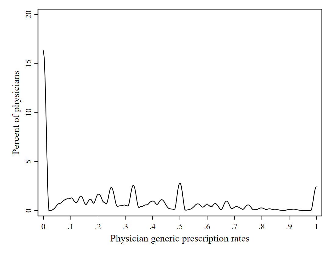
Figure 5.1: Hellerstein Figure 1 - Distribution of Physician Generic Prescription Rates (Source: NAMSCd91)
5.4.1.5 Figure 2
We only keep physicians that prescribe the same multisource drug to at least six patients, independent of whether it is in its generic or trade-name form. We compute the mean of the generic share for each remaining physician and create a categorical variable on whether this mean is 0, indicating only trade-name drugs; 1, indicating a mix of generic and brand-name versions; or 2, indicating only generic drugs. We plot the frequencies of these three categories across physicians in a bar plot (Section 8.2).
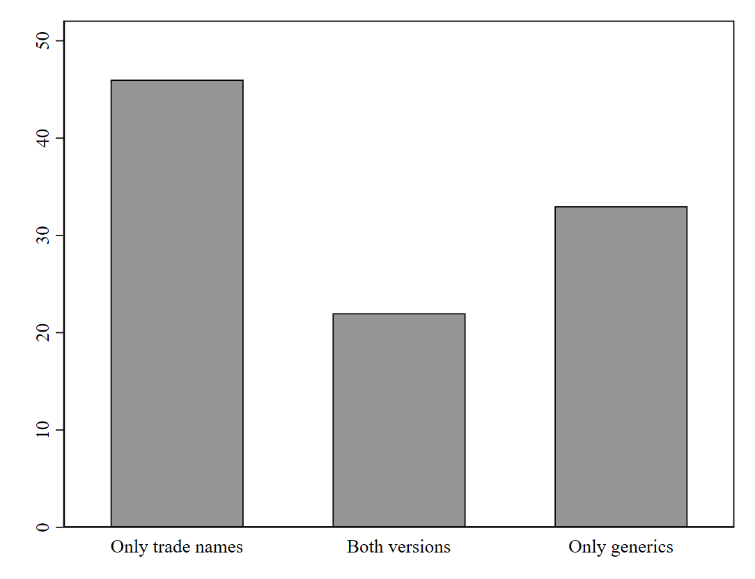
Figure 5.2: Hellerstein Figure 2 - Physician decisions by physicians who prescribe a drug to at least six patients (Source: NAMSCd91)
5.4.2 Generate estimates of your investigated effect using regression techniques
Hellerstein applies a random effects probit regression model aggregated on physician level. The parameterization of the model is implemented as follows:
Dependent variable (\(Y\))
- \(G\): Generic compared to brand-name drug use
Note that Hellerstein uses a somewhat different notation for the outcome variable which is denoted as \(G\). Today, it is common to denote this variable by \(Y\).
Variable of interest or treatment (\(X\))
- \(P\): Insurance status by: Medicare, Medicaid, HMO/prepaid, private insurance, self-paid (this is the omitted category).
Note that Hellerstein (1998) uses a somewhat different notation for the variable of interest which is denoted as \(P\). Today, it is common to denote this variable by \(X\) or \(D\). Though for the purpose of the reproduction and to avoid confusion we take on Hellerstein’s notation in the following.
Confounders \(Z\) of the effect of insurance status \(P\) and generic vs brand-name drug use \(Y\).
- \(C\): Drug class identifiers among 8 classes (Pain relief (omitted), see footnote Table 5)
- \(X\): Patient characteristics: age, sex, race
- \(S\): Physician specialist status: Specialist, general practitioner (omitted)
- \(R\): Region as classified by: Midwest, South, West, Northeast (omitted)
- Vector \(X\) Average patient characteristics in one practice
- Vector \(P\): Average of a physician’s patients in each insurance category
Note that Hellerstein uses a somewhat different notation for confounding variables. It is common to denote the variable of interest using the index \(X\), but not necessarily confounders.
5.4.2.1 Tables 4 and 5
We estimate the regression coefficients, t-statistics and marginal effects of the regression model. It is not indicated whether the model for both tables contain all covariates specified in equation 10 or just the variables mentioned in the tables. We decide to use the full model for both tables. Marginal effects are the average marginal effects across individuals (footnote Table 4) (Section 8.3).
Hellerstein Table 4 - Estimated Coefficients on Demographic Variables, Geographic Variables, and Average Characteristics for Full Sample, excluding regional identifiers
| Random-Effects Probit Coefficient | % Change in Generic | |||
|---|---|---|---|---|
| Constant | -0.556** | (-3.17) | ||
| Age | -0.002* | (-1.99) | -0.001* | (-1.99) |
| Female | -0.112** | (-2.94) | -0.028** | (-2.94) |
| Hispanic | 0.025 | (0.28) | 0.006 | (0.28) |
| Nonwhite | 0.044 | (0.62) | 0.011 | (0.62) |
| Specialist | 0.019 | (0.25) | 0.005 | (0.25) |
| Mean age | -0.003 | (-1.10) | -0.001 | (-1.10) |
| Percent female | -0.189 | (-1.16) | -0.048 | (-1.16) |
| Percent black | 0.075 | (0.41) | 0.019 | (0.41) |
| Percent Hispanic | -0.112 | (-0.45) | -0.028 | (-0.45) |
| Percent Medicaid | 0.062 | (0.26) | 0.016 | (0.26) |
| Percent Medicare | -0.155 | (-0.71) | -0.039 | (-0.71) |
| Percent private insured | 0.155 | (1.08) | 0.039 | (1.08) |
| Percent HMO/prepaid | 0.054 | (0.30) | 0.014 | (0.30) |
| Midwest | -0.141 | (-1.53) | -0.036 | (-1.53) |
| South | -0.206* | (-2.28) | -0.052* | (-2.29) |
| West | 0.065 | (0.67) | 0.016 | (0.67) |
Notes: \(*p < 0.05, **p < 0.01, ***p < 0.001\). The sample size is 7,715. For further notes see Hellerstein (1998). Data source: NAMSCd91.
Table 5 shows the estimated coefficients for the eight largest drug classes as well as the percentage change in the generic share. The greatest difference compared to Hellerstein (1998) is the change in sign from positive to negative for cardiovascular/renals, though not significant in our model.
Hellerstein Table 5 - Estimated Coefficients for Drug-Class Dummy Variable for Full Sample
| Random-Effects Probit Coefficient | % Change in Generic | |||
|---|---|---|---|---|
| main | ||||
| Antimicrobials | 0.628*** | (8.47) | 0.159*** | (8.54) |
| Cardiovascular-renals | -0.147 | (-1.71) | -0.0371 | (-1.71) |
| Central Nervous System | 0.0559 | (0.58) | 0.0141 | (0.58) |
| Hormones/Hormonal mechanisms | 0.584*** | (6.92) | 0.148*** | (6.95) |
| Skin/Mucous membrane | -0.731*** | (-6.26) | -0.185*** | (-6.28) |
| Ophthalmics | -0.383* | (-2.47) | -0.0968* | (-2.47) |
| Resperatory tract | -0.675*** | (-4.79) | -0.171*** | (-4.80) |
Notes: \(*p < 0.05, **p < 0.01, ***p < 0.001\). The sample size is 7,715. Omitted category is pain relief. For further notes see Hellerstein (1998). Data source: NAMSCd91.
5.4.2.2 Table 6
We run a separate regression using only observations of a single drug class and report the coefficients of the payment dummies and their average marginal effects (Section 8.2).
Hellerstein Table 6 - Tests for Moral Hazard for the Full Sample Equality of Individual Insurance Variables with Self-Payment Random-Effects Probit Results
| Antimicrobial | % change | Cardiovasculars | % change | Central Nervous System | % change | Hormones | % change | Skin/Muchous Membranes | % change | Ophthalmics | % change | Pain relief | % change | Respiratory Tract | % change | |
|---|---|---|---|---|---|---|---|---|---|---|---|---|---|---|---|---|
| Medicaid | ||||||||||||||||
| Coefficient | 0.14 | 0.04 | 0.00 | 0.00 | 0.02 | 0.00 | 0.38 | 0.08 | 0.03 | 0.00 | -0.25 | -0.05 | 0.54 | 0.08 | -1.21 | -0.09 |
| 1.12 | 1.13 | 0.02 | 0.02 | 0.08 | 0.08 | 1.23 | 1.23 | 0.04 | 0.04 | -0.60 | -0.60 | 1.12 | 1.15 | -1.08 | -1.11 | |
| Medicare | ||||||||||||||||
| Coefficient | 0.11 | 0.03 | 0.05 | 0.01 | -0.32 | -0.06 | -0.42 | -0.09 | 0.54 | 0.05 | -0.41 | -0.08 | 0.08 | 0.01 | -0.60 | -0.05 |
| 0.72 | 0.72 | 0.25 | 0.25 | -1.13 | -1.12 | -1.68 | -1.69 | 0.89 | 0.90 | -0.97 | -0.97 | 0.18 | 0.18 | -0.67 | -0.68 | |
| Private | ||||||||||||||||
| Coefficient | 0.00 | 0.00 | -0.06 | -0.01 | -0.06 | -0.01 | -0.16 | -0.03 | 0.03 | 0.00 | -0.31 | -0.06 | 0.18 | 0.03 | -1.27 | -0.10 |
| 0.01 | 0.01 | -0.30 | -0.30 | -0.28 | -0.28 | -0.75 | -0.75 | 0.07 | 0.07 | -0.91 | -0.91 | 0.51 | 0.51 | -1.45 | -1.56 | |
| HMO/Prepaid | ||||||||||||||||
| Coefficient | 0.22 | 0.06 | -0.14 | -0.03 | 0.32 | 0.06 | -0.33 | -0.07 | -0.42 | -0.04 | -0.57 | -0.11 | 0.28 | 0.04 | -0.26 | -0.02 |
| 1.78 | 1.78 | -0.56 | -0.56 | 1.04 | 1.05 | -1.09 | -1.09 | -0.73 | -0.73 | -0.93 | -0.93 | 0.71 | 0.72 | -0.26 | -0.25 |
Notes: see Hellerstein (1998). Data source: NAMSCd91.
5.4.2.3 Tables 7, 8 and 9
These tables cannot be reproduced as the publicly available data of NACMSd do not provide variables to identify physicians and patients by region.